• home
• writing
• research

Models of synaptic conductance II

NOTE  In this set of articles I would like to cover three simple models of synaptic conductance which are typically used in spiking networks. While people are quite familiar with their general logic, the exact mathematical details are often overlooked or simply swept under the rug because they are deemed too simple. I will take on this all-too-simple task, and talk about the mathematical ideas behind these basic models.

In the first article of this series we discussed synapses which activate instantaneously. These synapses are easy to program, and offer an excellent approximation when one is interested in phenomena occurring at timescales larger than the activation dynamics. However, once we go down to about we typically want to take the activation dynamics into account. In this article, we look at a common, first-approximation to such transfer functions - the alpha function:

Here, is the conductance and is the time-scale constant which describes both the rise and the fall of the electric flux. Of course, we are assuming there is no external perturbation from onwards. This is illustrated in the figure below for and . Notice that equation is normalised such that the response peaks at and the amplitude at the peak is .

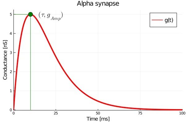
To gain a better intuition about the behaviour of the alpha synapse, let us try to formulate its equations of motion. A first attempt makes it clear that a single state variable does not suffice, i.e., it is not as ‘memoryless’ as the ISED synapse. However, after some manipulation one can arrive at:

We have introduced a second variable which describes a decay function reminiscent of the ISED equation. The conductance can then be said to simply follow this trace variable as if it were a dynamic fixed-point which itself was converging to zero. This gives us a two-dimensional state with a fixed point at . A simple analysis of equation reveals that this fixed point is a degenerate node. Some trajectories of this system with are shown below.

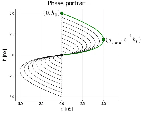
There are a few things to note here. First, I have only plotted the first and third quadrants as synapses cannot be both excitatory and inhibitory. Second, the sense of all trajectories is towards the origin (black circle) - this is not evident from the plot. For most trajectories, the conductance (i.e., the abscissa) grows, attains a maximum amplitude, and then decays to zero. Furthermore, given a trajectory , this amplitude () has exactly the same value as the non-zero vertical intercept (say, ) of the trajectory. This is illustrated in the figure above using the green trajectory, where two green circles are used to mark the vertical intercept and the maximum amplitude. We verify that, indeed, ( for this particular trajectory) - a very useful property of the system, as we shall see below.

Now for the spiking. What do you think happens when the synapse receives another pre-synaptic spike while the conductance is still non-zero? Ideally, one would want the system to not only reset, but to also remember the impact from the previous inputs. In ISED synapses, this memory is not needed as the impact is instantaneous. However, in alpha synapses this memory is crucial, and can be implemented by a simple extension of equation :

Here, the pre-synaptic spike (arriving at ) leads to an eventual increase in the conductance by . The increase is modelled by an instantaneous jump in , which causes the synapse to hop to a trajectory with a higher amplitude. However, this discrete ‘hop’ is not reflected in the conductance , which changes smoothly. It can only be observed in the future. Note that in equation , since for any trajectory (as shown above), the discrete ‘hop’ in has the effect of moving the synapse to a trajectory which corresponds to an additively updated maximum amplitude. In the figure below, I show the effect of a volley of input spikes on the conductance of an alpha synapse.

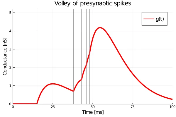
Here, the arrival times of the input spikes are shown using grey vertical lines, and each input spike has . Notice how, after each input spike, the conductance takes off on a steeper, upward trajectory.

The alpha synapse offers an excellent first approximation of the synaptic activation dynamics, and suffices for most simulations. However, it assumes equivalent time-scales for both the rise and the decay of the impulse response - something that may not be desirable when one wants to model specific transfer functions in detail. In the next and final article of the series, we will look at a second approximation of the synaptic transfer function which tries to address this problem.